Video Tutorials

There are three ways to download the xmeta package in R:

  1. ​Go to Packages tab on bottom right quadrant of R. Scroll through the options and select xmeta.
  2. ​Type: install.packages(“xmeta”). Then, to download the packaged for access, type: library(“xmeta”).
  3. ​Click on the Tools tab in your Menu bar, which is at the top of your computer screen. Go to the Install Packages option and type in the empty text box or scroll to select xmeta. Once installed, type: library(“xmeta”).

In this tutorial, we briefly introduce the xmeta package and its main functions.

  1. X-meta denotes “a toolbox for multivariate meta-analysis”.
  2. This package includes a collectin of functions:
    • The mmeta function: making inference in multivariate meta-analysis. The aim of the function is to estimate the underlying pooled effects and the components of the between-study covariance matrix for multivariate random-effects meta-analysis.
    • The SSE function: detecting and quantifying small study effects (SSE), which include publication bias, in multivariate meta-analysis. This function implementing the multivariate Egger’s regression test and multivariate trim and fill method for detecting SSE, as well as a novel method to quantify SSE.
    • The galaxy function: visualizing features of multivariate meta-analysis. This function implementing the the commonly used visualization tools for meta-analysis, including the forest plot, the bubble plot, the SROC curve, the cross-hairs plot, and the galaxy plot. The galaxy plot is a novel visualization tool for MMA, which preserves all information contained in two separate funnel plots in a two-dimentional space.

We are going to talk about more details about the three main function in later tutorials.

Tutorial 3.0: Introducing the mmeta Function

The mmeta function can be used to perform multivariate random-effects meta-analysis for binary or continuous datasets. The structure of the mmeta command is the same for both types of data, though the estimation methods differ.

Tutorial 3.1: Using mmeta Function for Continuous Data

For continuous data, the estimation methods that can be used are nn.reml, nn.cl, nn.mom, and nn.rs, where nn refers to the bivariate random-effects meta-analysis model.

Tutorial 3.2: Using mmeta Function for Binary Data

For binary data, the estimation methods that can be used are bb.cl, bn.cl, tb.cl, and tn.cl. These methods all use the composite likelihood estimator and correspond with different distributions: beta-binomial, bivariate-normal, trivariate-beta, and trivariate-normal, respectively.

Tutorial 4.1: Galaxy plot in XMETA

The Galaxy plot provides a new method for displaying the information found in the funnel plot by creating one-dimensional and two-dimensional plots.

To aid in the visualization, we first reduce the dimension of a univariate funnel plot as demonstrated in the left panel of this figure. The main idea is to project the two-dimensional univariate funnel plot (i.e., effect size and standard error are displayed using two axes) to the one-dimensional galaxy plot. The one-dimensional Galaxy plot represents the effect size and standard error data points using circles on an axis. The axis is a continuum for effect size while the size of the circles on the axis corresponds with that study’s precision. Larger studies, and thus studies that are more precise, are represented by bigger circles. The size of each circle coincides with its contribution to the weighted sum estimate of the overall effect size. We can obtain a high-level view of where the effect sizes of different studies fall relative to each other through the one-dimensional galaxy plot .

The two-dimensional Galaxy plot incorporates a similar visualization technique and can be used to compare two outcomes. The x and y axes of the Galaxy plot are the two different outcomes being studied. Within the plane, each study is represented by an ellipse whose location and size are determined by the point estimates and precision (inverse of standard error) of the two outcomes. The crosshair in each ellipse helps to display the precision, and its intersection shows the estimate of the bivariate outcomes. The center of mass of the galaxy, which is marked by the red star among the ellipses, corresponds to the overall estimate of the two outcomes.

We term these as Galaxy plots for their similarity to images of galaxies.

Tutorial 4.2: Visualizing Specific Features Using Galaxy Plot

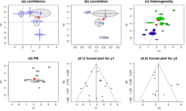
(a). Galaxy-confidence plot:
The galaxy-confidence plot uses cross-hairs to represent the confidence intervals with the cross point showing the point estimate of the bivariate outcome. The confidence intervals are then compared with the lines representing no effect (i.e., black dash lines) to help determine the significance of the effect sizes.

​(b). Galaxy-correlation plot:
The galaxy-correlation plot displays the within-study correlation of each individual study by an arrow starting from the center of the ellipse. We restrict the range of arrow to the right side of the ellipse, and the range of correlation (-1, 1) is mapped to the radian range (an arrow above the x-axis represents a positive correlation, while one below the x-axis represents a negative correlation).

​(c). Galaxy-heterogeneity plot:
TThe galaxy-heterogeneity plot enables investigations of heterogeneity in a bivariate space. For example, the ellipses in green represent the studies comparing Treatment A and the placebo, while the ellipses in blue represent the studies comparing Treatment B and the placebo.

​(d). PB investigation:
In the presence of PB, the galaxy plot is usually not symmetric around the estimated center of mass. More sophisticated statistical methods to quantify and correct for PB can be developed based on this Galaxy plot.


Egger's Test

Focusing on funnel plot symmetry, Egger et al. (1997) used a simple but effective regression-based test to detect PB. Specifically, they proposed to regress the standardized effect size (i.e., the effect size divided by its standard error) against precision and then test for nullity of the intercept. In the case of no PB, the intercept of the regression line should be zero, while if PB is present, the intercept deviates from zero due to the asymmetry. There are several variations of Egger’s test in the framework of univariate meta-analysis. Macaskill et al. (2001) introduced a different regression approach to detect PB, where the effect size is regressed on sample size of the study with weights being the inverse of the variances. A similar approach was suggested by Peters et al. (2006), where the sample size is replaced by its inverse.

# Egger's linear regression test

ms1 <- metabin(Ee, Ne, Ec, Nc, data=data1)
summary(ms1)
funnel(ms1)

metabias(ms1, method="linreg")
reg <- lm(I(ms1$TE/ms1$seTE)~I(1/ms1$seTE))
summary(reg)
radial(ms1)
abline(reg)

Begg's Test

Begg and Mazumdar (1994) proposed a nonparametric rank correlation method for PB based on Kendall’s tau. Their method tests whether the standardized effect size and the variance of the effect size are significantly associated. An estimated Kendall’s tau rank correlation coefficient that is close to zero indicates a high degree of independence between the variance and the standardized effect size, suggesting the absence of PB. On the other hand, an estimated Kendall’s tau rank correlation coefficient that is significantly greater than zero indicates the presence of PB. Possible variations of Begg’s rank test can be obtained by replacing standard errors by the inverse of total sample size. However, Begg’s rank test may be underpowered if the number of studies in a meta-analysis is only moderate (Sterne et al., 2000).

# Begg's rank-correlation test

ms1 <- metabin(Ee, Ne, Ec, Nc, data=data1)
summary(ms1)
funnel(ms1)

metabias(ms1, method="rank")

Trim and Fill Method

The Trim and Fill method is a popular nonparametric method to detect and correct for PB. The idea behind this method is to add studies to an asymmetric funnel plot until it becomes symmetric. Duval and Tweedie proposed three estimators of the number of missing studies (Duval and Tweedie, 2000). Under the null hypothesis, the approximate distributions of the three estimators were derived and can be used to test for PB.

# Trim-fill method

ms1 <- metabin(Ee, Ne, Ec, Nc, data=data1)
summary(ms1)
funnel(ms1)

tf1 <- trimfill(ms1)
class(tf1)
funnel(tf1)
print(tf1,digits=2,comb.fixed=TRUE)